This new study investigates what other information we can extract from satellite radar altimetry measurements of the Greenland ice sheet in addition to changes in the surface elevation. Specifically, we want to know if the strength with which radar signals are reflected from the ice surface can be related to properties of that surface, namely its density and roughness; important things to know if we want to make accurate predictions of how Greenland will evolve with climate change. A useful analogy for how we approach this would be to think about how light from a flashlight reflects from different surfaces; a reflection from a mirror will look much brighter than a reflection from a carpet. It is similar type of analysis we apply to Greenland, only with different radar altimeters standing in as our flashlight.
The technique we use (Radar Statistical Reconnaissance) was initially developed to study the surface of Mars but has also been used to study Earth’s ice sheets as well as Saturn’s moon Titan. Through RSR, we can separate how “mirror”-like (i.e., coherent) the surface of Greenland is from how “carpet”-like (i.e., incoherent) it is. With a prediction of how radar energy reflects from a surface, we can then use the strength of the “mirror”- and “carpet”-like components to estimate the density and roughness.
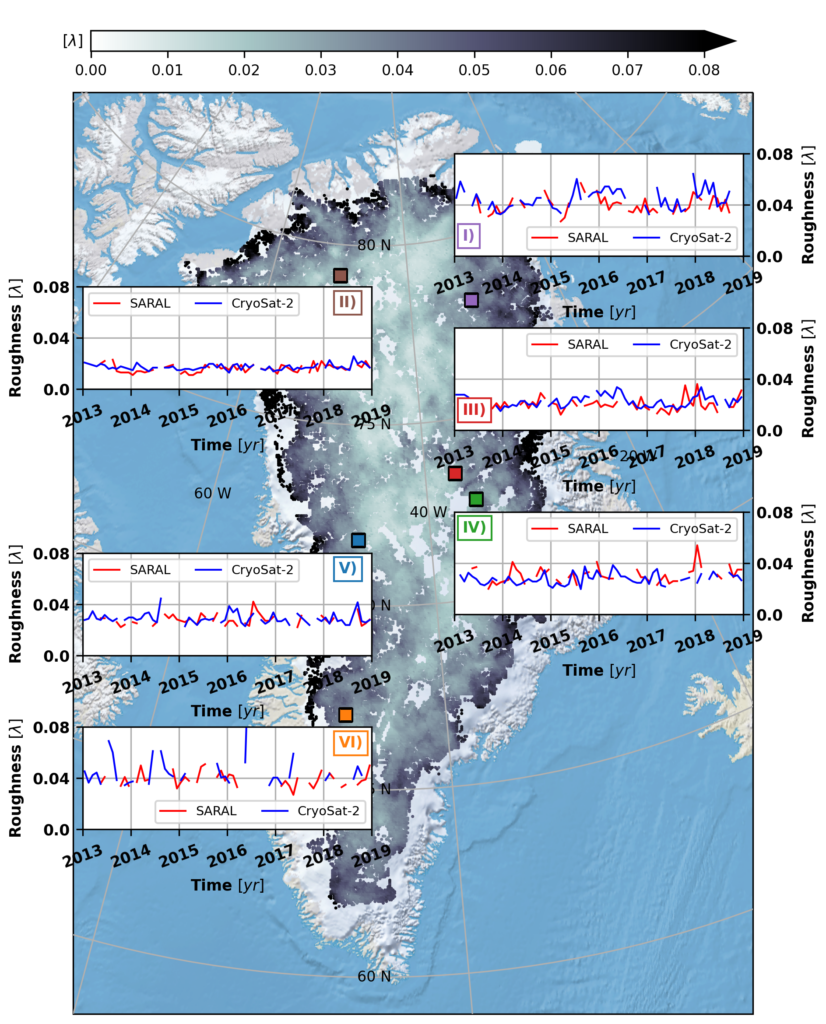
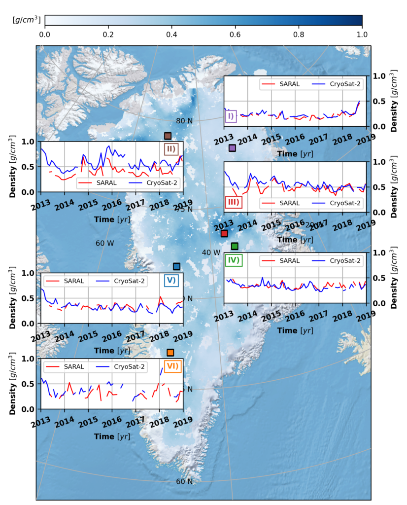
Our timeseries and maps of density and roughness tell us how the surface of Greenland changed between January 2013 and December 2018. For the latter, surface roughness hasn’t changed so much with time, but seems tightly associated to ice flow speeds (i.e., where the ice flows faster, the surface is rougher). In terms of the former, density seems strongly affected by extremely warm summers (e.g., 2012 everywhere and 2015 in NW Greenland) before eventually returning to consistent levels. This result, and how it differs between our two different radar “flashlights” (ESA CryoSat-2, CNES/ISRO SARAL), leads us to think that we can, at least in a qualitative sense, measure how density changes with depth in the near-surface. Our CryoSat-2 “flashlight” seems to see a little deeper into the near-surface than SARAL, since CryoSat-2 densities are almost always greater, and the dense layers formed after summer melting take longer to be deeply buried by subsequent snowfall.
Overall, looking into how strongly radar signals are reflected from the surface of Greenland gives us new observations into how it responds in a changing climate. These observations are critical parameters in evaluating Greenland’s on-going contribution to global mean sea-level rise.
Greenland surface density (May 2015 SARAL basemap)
Full Study
Scanlan, K. M., Rutishauser, A., & Simonsen, S. B. (2023). Observing the near-surface properties of the Greenland ice sheet. Geophysical Research Letters, 50, e2022GL101702. https://doi. org/10.1029/2022GL101702
Information about the sea ice surface topography and related deformation are crucial for studies of sea ice mass balance, sea ice modeling, and ship navigation through the ice pack. Spaceborne altimeters are able to derive estimates of the sea ice topography, identify leads (fractures in the ice with calm open water, representative of the local sea level), and provide a measure of the sea ice thickness distribution – but, at what resolution? This study aims to assess the capabilities and uncertainties of NASA’s high-resolution spaceborne laser altimeter, Ice, Cloud, and land Elevation Satellite-2 (ICESat-2), by comparing with coincident helicopterborne laser scanner observations achieved during the Multidisciplinary drifting Observatory for the Study of Arctic Climate (MOSAiC) Expedition in the Arctic Ocean. The goal is to investigate how the sea ice surface roughness and topography is represented in different ICESat-2 products, and how sensitive ICESat-2 products are to leads and small cracks in the ice cover. The study was co-lead by Dr. Robert Ricker from NORCE and Dr. Steven Fons at NASA Goddard Space Flight Center and the University of Maryland. It was a collaboration across several institutes working with Arctic sea ice and altimetry, here amongst DTU Space, and the study was recently published in The Cryosphere.
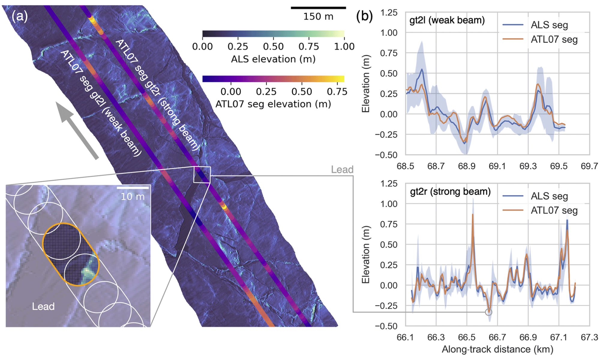
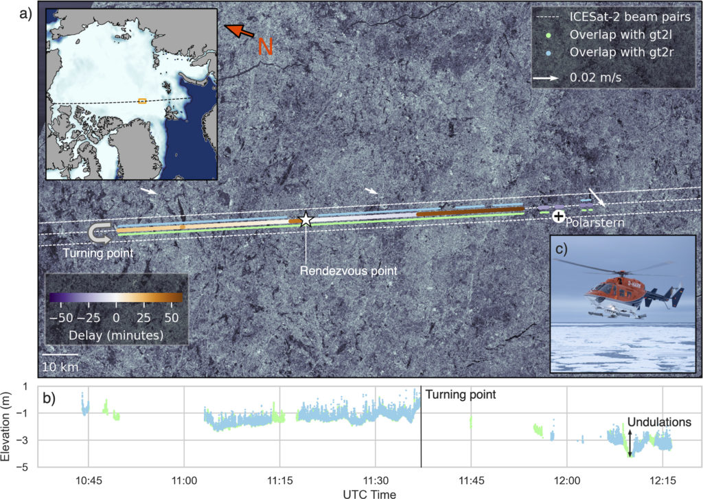
Overview of the helicopter flight and airborne measurements coincident with ICESat-2 underflight (Ricker et al., 2023). See the original article for a full figure caption.
Here, we present a new validation data set for ICESat-2 sea ice measurements that was acquired during the MOSAiC campaign (Nicolaus et al., 2022). The helicopter aboard the drifting research vessel (RV) Polarstern was equipped with an airborne laser scanner (ALS). On 23 March 2020, they followed an ICESat-2 ground track in close vicinity for 130 km. The ALS data was compared with two ICESat-2 surface elevation datasets (computed using different algorithms; the operational NASA product (ATL07) and the high-fidelity product of the University of Maryland, UMD) to investigate the limitations and capabilities of the different algorithms and the spaceborne data. The ALS data was drift-corrected (based on highest correlation) and the comparisons incldes the ALS data at full resolution, the ALS data sampled to ALT07 resolution as well as ATL07 and UMD at their respective resolutions. In this comparison and evaluation of the ICESat-2 observations, the study primarily focused on the ability to detect and estimate the magnitude of sea ice obstacles (assumed to be pressure ridges), the impact of sea ice roughness, and the ability to detect leads. Below we shall summarize some of the main findings of the study.
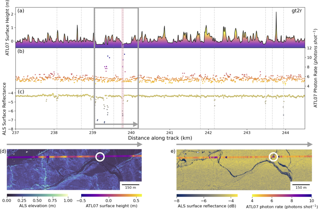
One lead was identified in the ATL07 observations of the strong beam of ICESat-2 (no leads identified in teh weak beam). Here, a comparison of ATL07 surface elevations, ICESat-2 ATL07 photon rates and ALS surface reflectance are shown along a 7 km transect during the underflight.
Lead identifications While the segment shown was relatively short (~7 km), only 1 of 10 leads identified in ALS was also identified in ATL07. This contrast between ALS-identified leads and ATL07-identified leads is remarkable. From the ATL07 photon rate and surface height, we observe potential leads that were not classified as such, including those between kilometers 243 and 244. Reasons for this could include the leads observed along this profile mostly being very small (only few meters wide), refrozen cracks in the ice. These cracks are smaller than the ICESat-2 footprint and much smaller than the 150-photon-aggregate segments; therefore, the elevations and photon rates get smoothed by the surrounding ice floes and do not meet the threshold criteria to be considered a lead. Another aspect that adds to the discrepancies comes from the fact that the ALS swath is wider than the ATL07 segment width and that the ALS lead-finding procedure incorporates returns from outside of the overlapping segments. Future analysis of overlapping profiles that flew over more, open, and larger leads would be better to assess the ATL07 parameter lead thresholds and determine the minimum detectable width of leads. Additionally, a future modification to the ATL07 algorithm could be implemented that, for example, relaxes the 150-photon requirement for leads, as fewer signal photons should be needed to get an accurate height retrieval over flat surfaces.
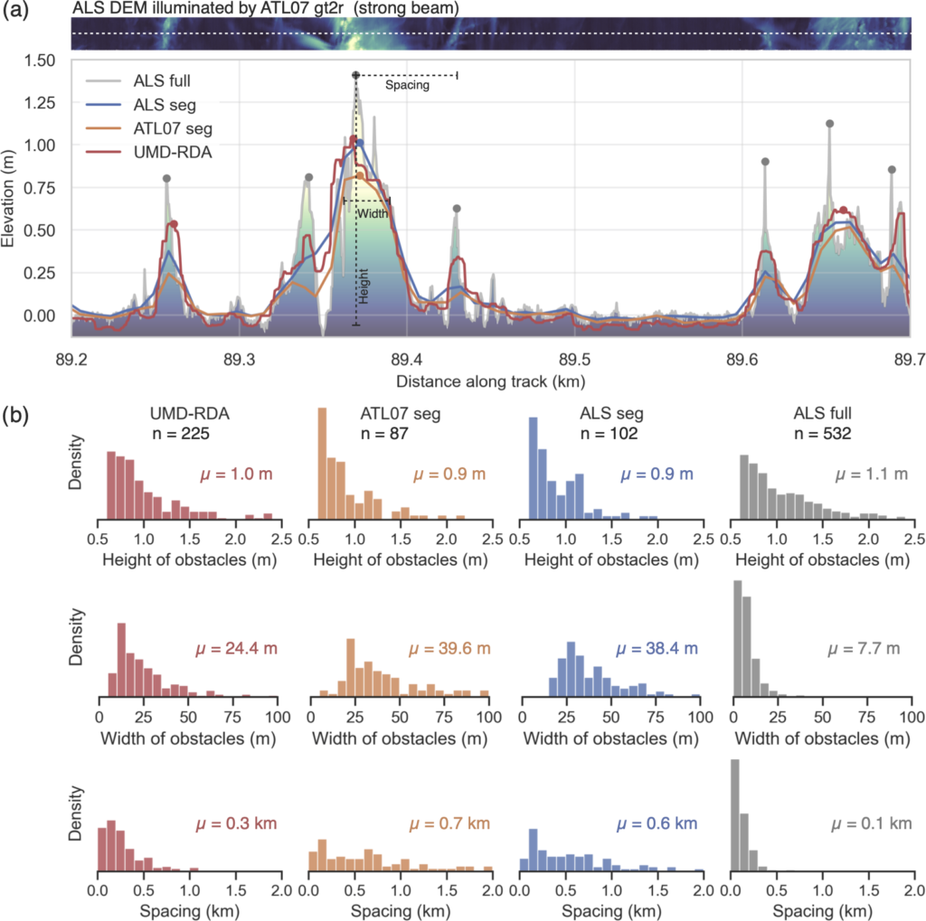
Surface elevations using ALS full resolution (ALS full), ALS sampled to ALT07 resolution (ALS seg), ATL07 and UMD observations, and with a ridge-detection algorithm (find peaks in data), identified obstacles and their statistics are provided.
Ridge detections Our results show that ICESat-2 allows for detection and height estimation of individual surface topography features. However, comparison with the high-resolution ALS data set also shows that not all ridges or obstacles will be captured. Ridge detection and sail height estimation depend on the applied algorithm, the dimensions of the ridge, and the data product used. While the height distributions of the detected ridges reveal similar shapes among all products, the width distributions differ substantially. The reason for this is that the width estimates strongly depend on the along-track resolution. The smoothing effect mentioned earlier leads to an increase in width, while narrow ridges with small widths (<5 m) can barely be detected with ATL07. The choice of segment length (ATL07 is of varying segment length using 150-photon aggregates, whereas UMD-RDA aims to provide observations on a per-shot basis) is also a choice made based on the overall objective of each algorithm. While ATL07 aims to provide observations of the average local sea ice elevation, UMD-RDA aims to sample the top of the sea ice pressure ridges. Therefore, UMD-RDA is more likely to provide higher estimates. The fact that neither ATL07 nor UMD-RDA is able to capture the full extent of the surface topography likely shows the limitations of ICESat-2 for specific obstacle detection. With that being said, considering that ICESat-2 is a spaceborne platform observing meter-scale features from a 500 km orbit, these results are remarkable if compared to previous satellite altimeter missions.
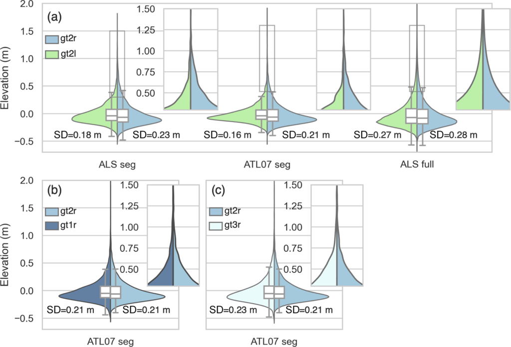
A comparison of surface elevations for ALS seg, ALS full and ATL07: comparing observations related to the strong (gtr) and weaks beams (gtl) of the center beam of ICESat-2 (gt2r/gt2l) which the helicopter was targeting, as well as the additional beam pairs of ICESat-2 (gt1r and gt3r).
Weak beams vs strong beams The differences between the weak and strong beams are a result of the surface reflectance and laser power, and with the laser power of the strong beams being about 4 times greater than that of the weak beams, the segments of the weak beam are about 3.5 times longer in order to collect the 150 signal photons. This results in smoother elevation profile for the weak beam, whereas the strong beam reveals more details of the surface topography. However, when comparing the aforementioned elevation profiles to segment-averaged ALS elevations, we find that the performance of the weak beam is comparable to the strong beam. Thus, weak-beam elevations are suitable for large-scale studies of the sea ice freeboard and thickness, when small-scale topography is less important.
Full study: Ricker, R., Fons, S., Jutila, A., Hutter, N., Duncan, K., Farrell, S. L., Kurtz, N. T., and Fredensborg Hansen, R. M.: Linking scales of sea ice surface topography: evaluation of ICESat-2 measurements with coincident helicopter laser scanning during MOSAiC, The Cryosphere, 17, 1411–1429, https://doi.org/10.5194/tc-17-1411-2023, 2023.
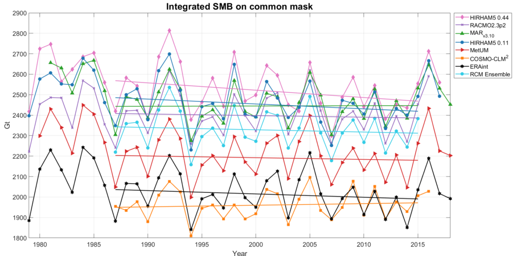
This study estimates the surface mass balance (SMB) of Antarctica, by making an intercomparison of five different regional climate models (RCMs) all simulating the Antarctic climate from 1987-2015. This study was led by Dr. Ruth Mottram from DMI and was a collaboration between several European institutes in Antarctic research, amongst other DTU Space and DMI, the study was published in The Cryosphere
The SMB is the sum of accumulation and ablation on an ice sheet surface. Accumulation is precipitation, which in Antarctica is primarily snowfall, and ablation consists of sublimation, evaporation, and runoff.
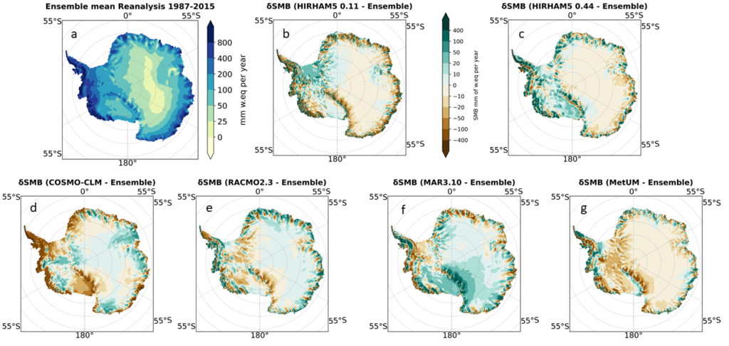
Our research shows that, when RCMs are forced by the ERA-Interim reanalysis data set, the integrated Antarctic ice sheet ensemble mean annual SMB is 2329 ± 94 Gigatonnes (Gt) per year. However, individual model estimates vary from 1961±70 to 2519±118 Gt per year, this spread corresponds to approximately 2 mm of global sea level per year. The large differences are mostly explained by different SMB estimates in West Antarctica and over the Antarctic Peninsula. Integrated over the continent all the RCMs show a consistent interannual variability, which is strongly correlated with the forcing data ERA-interim. In the interior of East Antarctica, the annual mean SMB is below 25 mm of water equivalent per year, in West Antarctica, it is greater than 1500 mm water equivalent per year. To evaluate the individual model performances of simulating near-surface climate, we have used in situ measurements of near-surface temperature, firn temperature, surface pressure, wind speeds, and SMB measurements. No one model outperforms the others, the models have different strengths and weaknesses for different variables in different regions. However, in areas with complex topography, e.g in West Antarctica and the Antarctic Peninsula the resolution of the models is extremely important, the higher resolution is, the better the topography is resolved, leading to changes in orographic precipitation and katabatic winds.
Annually resolved SMB integrated over the entire ice sheet for the different RCMs, in the period 1979-2018. All RCMs are driven by ERA-Interim and except for MARv3.10 and RACMO2.3p2, SMB is calculated according to Equation 1. The ensemble is a mean calculated from all 6 RCMs in the period 1987-2015 where there is data from all the models. All trend lines are calculated for the period 1987-2015.Sub-figure a show the SMB ensemble mean for the common period. Sub-figure b-g shows the difference between each model and the ensemble mean.
Full study: Mottram, R., Hansen, N., Kittel, C., van Wessem, M., Agosta, C., Amory, C., Boberg, F., van de Berg, W. J., Fettweis, X., Gossart, A., van Lipzig, N. P. M., van Meijgaard, E., Orr, A., Phillips, T., Webster, S., Simonsen, S. B., and Souverijns, N.: What is the Surface Mass Balance of Antarctica? An Intercomparison of Regional Climate Model Estimates, The Cryosphere, https://doi.org/10.5194/tc-15-3751-2021
The inland ice sheet that covers Greenland is shrinking and the melting is happening faster. This is confirmed by a new, detailed study carried out by researchers in the Department of Geodesy and Earth Observation, led by senior researcher Sebastian Bjerregaard Simonsen. The new research was recently published in the journal Geophysical Research Letters.
Research shows that from 1992 to 2020, more than 4,400 Gigatons of ice melted away. This melted ice has contributed to a 12 mm increase in the water level of the world’s oceans.
The research is based on altitude measurements over the 28 years with the ESA satellites ERS-1, ERS-2, ENVISAT, CryoSat-2 and Sentinel-3A. The unique thing about a new study is that the satellites cover the entire period with an uninterrupted time series and are based on the same measurement methods year by year. The Danish research team is the first to translate the long European time series of height changes into mass loss.
“On average, this corresponds to 158 Gigatons of ice melting each year over this period of nearly three decades. But there are big differences during the period and a clear trend towards the melting accelerating,” says Sebastian Bjerregaard Simonsen.
In the 1990s, the average melting rate was 57 Gt ice/year. In the 2000s it was 163 Gt ice/year. And in the 2010s, the average was 241 Gt of ice/year.
Simonsen, S. B., Barletta, V. R., Colgan, W., & Sørensen, L. S. (2021). Greenland ice sheet mass balance (1992‐2020) from calibrated radar altimetry. Geophysical Research Letters, 48, e2020GL091216. https://doi.org/10.1029/2020GL091216
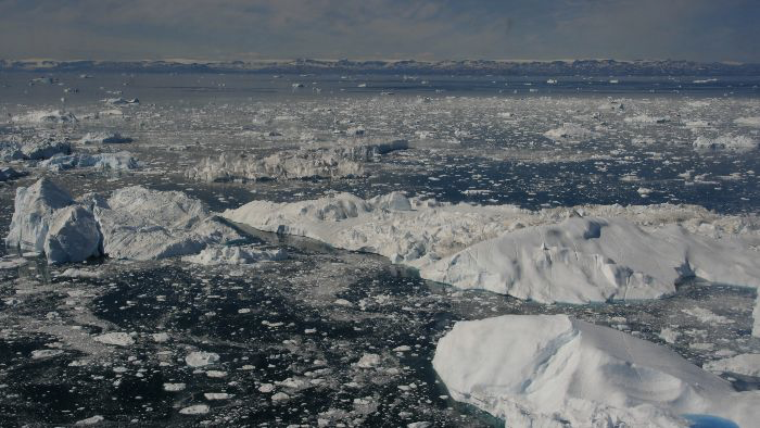
(Photo. Icebergs and large pieces of ice near Jakobshavn in Greenland. Photo: DTU Space/S.B. Simonsen)
We have just been involved in constraining the model range for firn model for the Greenland Ice sheet within the RETMIP project. The study was lead be GEUS and a summary of the findings is found below.
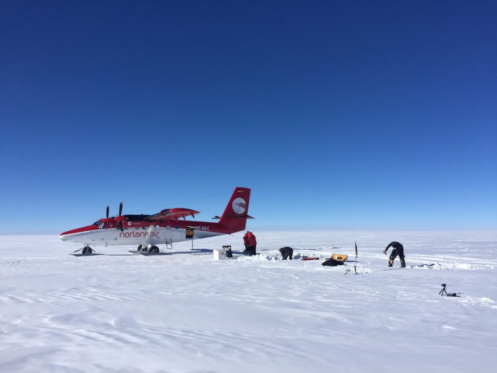
DTU Space conducting firn observations on the top of the Greenland Ice Sheet.
The thick snow that blankets the Greenland ice sheet provides a key service to the Earth’s system: the thick snow layer acts like a sponge when the surface of the ice sheet melts in the summer and prevents every year gigatons of meltwater to be poured into the ocean and contribute to sea-level rise. In a warming climate, we need computer models that can describe how this snow layer can retain meltwater generated at the surface of the ice sheet; and that is no easy task. Meltwater infiltrates and potentially refreezes in the snow depending on various parameters: the snow density and temperature, for example, or on how thick ice layers it contains. Multiple computer models are currently being used to simulate the retention of meltwater on the Greenland ice sheet. Yet, these models had never been evaluated on the same weather data input, until this new study.
A team of 23 researchers representing 18 research institutes and lead by Baptiste Vandecrux has evaluated nine snow models at four sites. These sites were chosen to represent the various climate present at the surface of the ice sheet: from cold and low-snowfall areas to warm and high-snowfall areas. What they found was striking: the snow models agree relatively well in the absence of melt, but the more melt was generated at the surface, the more models disagreed on where the water should infiltrate, whether it should refreeze and be retained or whether it should initiate a downslope flow towards the margin of the ice sheet and the ocean. Luckily, such a comparison exercise allows the team of researchers to identify key issues that snow models should address in the future. This greater insight on how snow models retain or not meltwater will hopefully allow the improvement of these models and allow a more accurate estimation of the current and future contribution of the Greenland ice sheet to sea-level rise.
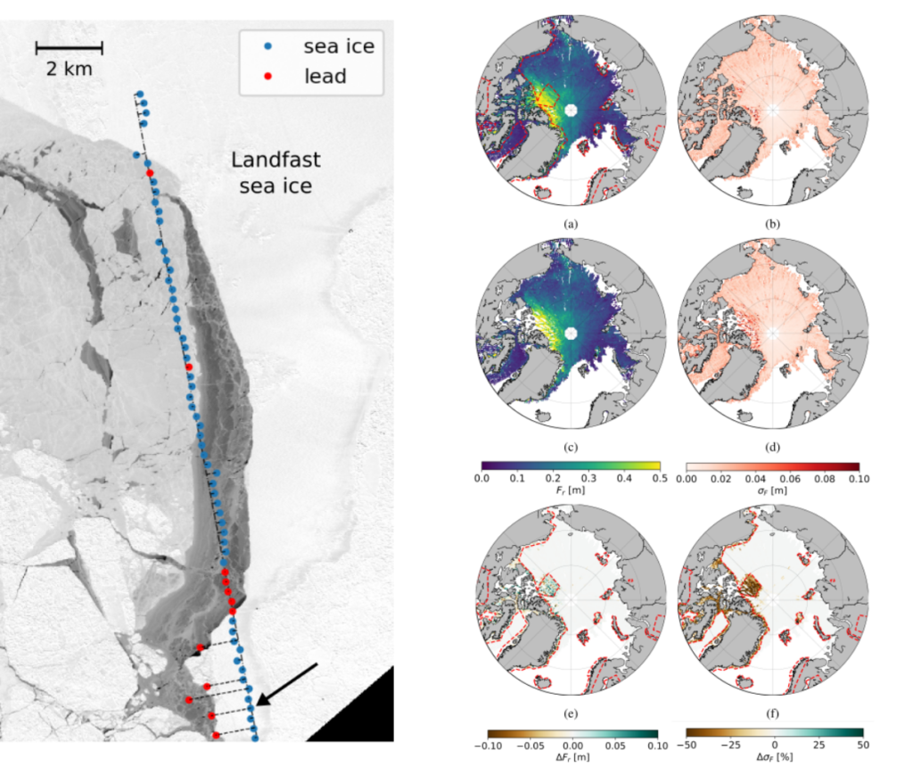
A new study by DTU Space and NASA JPL investigates the potential of performing “swath-like” processing of CryoSat-2 interferometric (SARIn) data over Arctic sea ice.
The proposed retracking method significantly increases the number of sea surface height retrievals, measured from leads, in the ice-covered Arctic Ocean reducing the uncertainty of sea ice thickness estimates from radar altimetry.
Left: In the lower part of the track, both sea ice and sea level elevations are extracted from single waveforms. Right: sea ice freeboard and corresponding random uncertainty in March 2014 from the swath-like algorithm (a, b) and a processor not using the SARIn phase information (c, d). (e) is the difference (a)–(c), and (f) represents the percentage of variation of (b) with respect to (d). Red dashed lines represent the boundaries of the CryoSat-2 SARIn acquisition mask. Source: https://doi.org/10.1109/TGRS.2020.3022522
This technique might potentially be applied to data from the Copernicus Polar Ice and Snow Topography Altimeter (CRISTAL) mission, due to launch in 2027. While CryoSat-2 measures the sea ice in SARIn mode only along the Arctic coastline, the instrument onboard CRISTAL is planned to operate in SARIn mode over the entire ice-covered region, and this method could provide high-density sampling of the sea level and the sea ice thickness in both the Arctic and Southern oceans.
Full study: Di Bella, Alessandro, Ronald Kwok, Thomas W. K. Armitage, Henriette Skourup, and Rene Forsberg. “Multi-Peak Retracking of CryoSat-2 SARIn Waveforms Over Arctic Sea Ice.” IEEE Transactions on Geoscience and Remote Sensing, 2020, 1–17. https://doi.org/10.1109/TGRS.2020.3022522.
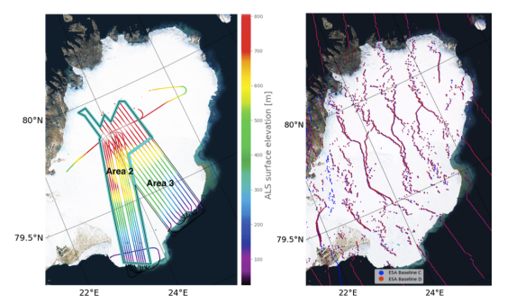
In connection to the development of the ESA Cryosat-2 baseline-D, we at EO4CRYO have been involved in the validation effort of the new product, based on our airborne surveys at Austfonna, Svalbard.
(left) The airborne elevation measurement from laser scanning. (Right) The differences in geolocation of the radar echo in the new and previous baselines.
How to cite and access the paper. Meloni, M., Bouffard, J., Parrinello, T., Dawson, G., Garnier, F., Helm, V., Di Bella, A., Hendricks, S., Ricker, R., Webb, E., Wright, B., Nielsen, K., Lee, S., Passaro, M., Scagliola, M., Simonsen, S. B., Sandberg Sørensen, L., Brockley, D., Baker, S., Fleury, S., Bamber, J., Maestri, L., Skourup, H., Forsberg, R., and Mizzi, L.: CryoSat Ice Baseline-D validation and evolutions, The Cryosphere, 14, 1889–1907, https://doi.org/10.5194/tc-14-1889-2020, 2020.